
 0
 EN
 English
 عربى
 Español
 русский
If you need any help, please feel free to contact us
Home / News / Industry News / Static Pressure vs Dynamic Pressure: What Flow Meter Selection Really Hinges On
Static Pressure vs Dynamic Pressure: What Flow Meter Selection Really Hinges On
A balancing contractor stands on a mezzanine with a pitot tube pushed through a duct wall. The reading is 0.42 inH2O. The commissioning engineer standing next to him insists the fan is delivering "plenty of static pressure" and the problem lies downstream. Both people are holding a number, and both are describing a different physical quantity with the same word: pressure. This is one of the most common and most expensive confusions in fluid measurement, because static pressure and dynamic pressure behave differently, are measured differently, and fail differently.
Here is the short answer before the detail: static pressure is the pressure the fluid exerts because it exists, and dynamic pressure is the pressure equivalent of the fluid's motion. They add up to total pressure, and almost every practical decision, from fan selection to orifice sizing to whether a gas meter needs temperature compensation, depends on knowing which of the three you are actually reading.
Static Pressure vs Dynamic Pressure: The Difference in One Sentence
Static pressure is stored energy per unit volume; dynamic pressure is kinetic energy per unit volume, expressed in the same units. Neither is more "correct" than the other. They are two entries in the same energy ledger, and the ledger has to balance.
For a fluid of density rho moving at velocity v, the dynamic pressure is:
q = 0.5 x rho x v squared
That is it. No correction factors, no empirical coefficients, no standard reference required. The simplicity is deceptive, because density is rarely constant in real processes, and velocity is exactly what most flow meters are trying to determine. The equation is also the source of one of the most useful diagnostic habits in instrumentation: if you know two of the three quantities, you can sanity check the third before you ever open a manual.
| Property | Static pressure | Dynamic pressure |
|---|---|---|
| Physical meaning | Stored, potential energy of the fluid; the pressure that acts on the pipe or duct wall | Kinetic energy per unit volume carried by the moving stream |
| Symbol and formula | p | q = 0.5 x rho x v squared |
| Direction | Acts equally in all directions at a point | Aligned with the flow direction; a scalar derived from a vector |
| Value at zero flow | Whatever the system pressure is, often several bar | Exactly zero |
| Typical measurement | Wall tap drilled perpendicular to the flow, or a static port on a pitot-static probe | Impact port facing the flow, or the difference between total and static pressure |
| Depends on density | Only through the fluid state | Linearly, which is why gas readings drift with temperature |
| Typical size, water line at 2 m/s | 3 to 10 bar in a process main | About 2 kPa (0.2 m of water) |
| Typical size, air duct at 8 m/s | 200 to 800 Pa | About 38 Pa |
Look at the last two rows. In a pressurised water main, the dynamic pressure is roughly four orders of magnitude smaller than the static pressure. In a low-pressure air duct, the two are the same order of magnitude. That single fact explains why a compressed air balancer works in inches of water while a pipeline engineer works in bar, and why the same instrument philosophy cannot be transplanted between the two worlds without adjustment.
Static Pressure: The Pressure That Does Not Need Motion
Static pressure is what a pressure gauge would read if it were drifting along with the fluid at the same velocity, undisturbed. In practice nobody floats a gauge down a pipe, so we approximate it with a wall tap drilled perpendicular to the axis of flow. The hole sees the fluid's random molecular motion but not its bulk forward momentum, and that is precisely the definition we want.
Three consequences follow, and each one causes field mistakes.
First, static pressure is not "the pressure when the fluid is stopped." A flowing pipe full of water at 6 bar has a static pressure of 6 bar while the water is moving at 3 m/s. The word static refers to the measurement frame, not to the fluid's state. Engineers who read it as "pressures only count when the pump is off" end up misdiagnosing cavitation, pump suction problems and blocked impellers.
Second, static pressure changes when velocity changes, even in a system with no friction. Push the same flow through a reducer and the static pressure drops in the narrow section while the velocity rises. This is the Bernoulli trade: total energy stays constant along a streamline, so what the fluid gains in motion it gives up in stored pressure. Venturi meters and flow nozzles are engineered around exactly this trade, which is why a well-made venturi recovers most of its pressure loss while an orifice plate does not.
Third, static pressure can be negative relative to atmosphere. A pump suction line running at minus 0.4 bar gauge is not an error; it is a system telling you the net positive suction head margin is thin and the fluid is close to flashing. Absolute and gauge references matter here, and a specification that says "0 to 10 bar" without stating the reference is an invitation to a warranty argument.
Dynamic Pressure: The Pressure Equivalent of Motion
Dynamic pressure is the pressure you feel when you hold your hand out of a moving car. The air is not at a higher static pressure; you are converting its forward momentum into a stagnation pressure on your palm. The conversion is complete and lossless at the stagnation point, which is why a pitot tube facing the flow reads total pressure and a static port reads static pressure, and the difference between them is the dynamic pressure.
Worked examples are more persuasive than formulas. Water at 1,000 kg per cubic metre flowing at 3 m/s produces a dynamic pressure of 4,500 Pa, or 4.5 kPa, or about 0.045 bar. Air at 1.2 kg per cubic metre flowing at 12 m/s produces just 86 Pa, less than 0.35 inH2O. The same velocity produces fifty times less dynamic pressure in air than in water because density differs by a factor of roughly 830.
This is the reason gas flow measurement is hard and liquid flow measurement is comparatively forgiving. A gas meter that derives flow from a differential pressure signal is working with a very small number, and that number moves with the square of velocity. At half the flow, the dynamic pressure falls to a quarter. At a tenth of the flow, it falls to one hundredth. Any fixed offset in the transmitter, any zero drift, any condensate leg in an impulse line, becomes a large percentage error at low flow.
Dynamic pressure appears in places far from instrumentation, which is a useful reminder of how general the concept is. Structural engineers size cladding and sign supports against q = 0.5 x rho x v squared for wind. Aerodynamicists speak of q as the driving quantity for lift and drag. HVAC engineers call it velocity pressure and use it to compute duct airflow from a pitot traverse. The formula is the same in all three; only the units and the tolerance change.
Total and Stagnation Pressure: Why the Sum Is What Many Sensors See
Total pressure is static plus dynamic. Stagnation pressure is the pressure at a point where the flow has been brought to rest isentropically; for incompressible flow the two terms are interchangeable, and for gases the difference is small below about Mach 0.3 and grows quickly above it.
A pitot-static probe is a two-in-one instrument. The forward-facing port sees total pressure. The side ports, set back far enough that the local flow is undisturbed, see static pressure. Plumb both to opposite sides of a differential transmitter and the signal is dynamic pressure directly. Plumb only the total port to a gauge and you have a stagnation pressure reading that is useless for flow unless you also know the static pressure.
Most field arguments about pitot tubes come down to which port was connected. A probe installed with the impact port at an angle, or a static port sitting in the wake of a weld, produces a reading that looks plausible and is wrong by 10 to 30 percent. Averaging pitot designs reduce this sensitivity by distributing multiple total and static ports across the pipe diameter, but they still depend on correct alignment; the manufacturer's alignment tolerance is usually a few degrees, not a few centimetres, and it is worth respecting.
How Each Pressure Is Measured in Practice
Static pressure taps are deceptively simple and routinely botched. The hole must be perpendicular to the wall, deburred, and free of burrs or gasket material protruding into the bore. A single tap in a pipe of small diameter reads high or low depending on the Reynolds number; the standards therefore specify multiple taps around the circumference, manifolded together, for anything above a certain size. Impulse lines must slope so that gas pockets or liquid slugs drain away from the transmitter, not into it.
Dynamic pressure measurement is more forgiving in principle and less forgiving in execution. The differential pressure generated is small, so the transmitter range is small, so the zero offset matters proportionally more. A 0.1 percent zero error on a 10 kPa span is 10 Pa, which is negligible; the same 0.1 percent on a 100 Pa span is 0.1 Pa, which is also negligible until you realise the span itself is only 100 Pa and the whole measurement is 1 percent of a typical industrial transmitter's range. High-rangeability, low-span transmitters exist for this reason, and so do dedicated low-differential sensors.
- Static taps: perpendicular, deburred, multiple taps manifolded on large lines.
- Total or impact port: directly facing the flow, aligned within a few degrees.
- Impulse lines: sloped, short, equal length on both legs, vented at the high point or drained at the low point.
- Transmitter: selected for span, not just for maximum rating; over-ranging destroys resolution.
- Temperature: a density assumption buried in a calculation is only as good as the temperature you actually measured.
Units, Square Roots and the Errors They Cause
Differential pressure flow elements produce a signal proportional to the square of flow. Invert that relationship and the error structure inverts with it. At 10 percent of full flow, a differential pressure element produces 1 percent of its span. If the transmitter has a fixed uncertainty of 0.1 percent of span, that uncertainty is 1 percent of reading at full flow and 10 percent of reading at 10 percent flow. This is not a fault in the instrument; it is arithmetic, and no amount of calibration removes it.
Practical turndown is therefore a procurement decision, not a commissioning discovery. A 5:1 turndown with a 1 percent reading requirement is achievable with a good differential transmitter and careful installation. A 20:1 turndown with the same accuracy requirement means you are specifying a different technology, not a better transmitter.
Unit confusion adds a second layer. Dynamic pressures in air are commonly quoted in inches of water, millimetres of water, pascals or pounds per square foot. One inch of water is about 249 Pa. A reading of 0.5 inH2O is 125 Pa. If a technician converts with the wrong factor, or with a factor that assumes a different reference temperature for water density, the error is a few percent, which is enough to fail a balancing specification but not enough to look obviously wrong on a screen.
There is also a habit worth breaking: comparing dynamic pressure readings taken at different fluid temperatures without correcting density. Air density changes about 0.35 percent per kelvin near ambient. A 20 K swing between a morning and afternoon test is a 7 percent density change and therefore a 7 percent flow error if the velocity pressure is converted with a fixed density. On a compliance test, that matters.
Compressible Flow: Where Static and Dynamic Pressure Diverge
Below Mach 0.3, treating a gas as incompressible costs about 2 percent in dynamic pressure, which is inside most process tolerances. Above that, the simple formula drifts, and by Mach 0.8 the gap is large enough to fail any serious measurement.
The isentropic relation links total and static pressure through the Mach number and the ratio of specific heats. For air with gamma of 1.4, the ratio of stagnation to static pressure is 1.89 at Mach 1.0 and 1.28 at Mach 0.6. In other words, at Mach 0.6 the dynamic pressure contribution is 28 percent of static pressure, and the "small correction" is no longer small.
This matters in compressed gas, steam and flare measurement far more often than people expect. A gas line at 20 bar and 20 m/s is only Mach 0.03, so compressibility is irrelevant to the pressure ratio, but the density is 20 times atmospheric and the dynamic pressure is correspondingly large. The compressor is not the issue; the density is. Conversely, a low-pressure steam line at 15 m/s is Mach 0.05 and still needs accurate density at operating temperature and pressure for the same reason.
Expansibility factors in standards such as ISO 5167 exist to handle exactly this. When a specification says "with expansibility correction," it is not adding paperwork; it is acknowledging that a gas accelerating through an orifice changes density, and that a differential pressure reading without the correction is systematically biased in one direction.
Static, Velocity and Total Pressure in Ducts and Air Handling
HVAC practice uses the same physics with different vocabulary, which is why cross-discipline conversations go wrong. Velocity pressure is dynamic pressure. Static pressure is the pressure acting on the duct wall. Total pressure is the sum. Fan curves are drawn in total pressure against flow, but selections are usually stated as external static pressure, which is the static pressure the fan must overcome in the attached system, excluding the fan's own internal losses.
Two practical rules follow from the definitions.
The first is that a fan does not "create static pressure." It adds total pressure across itself and, in a system with no change in velocity, almost all of that shows up as static. If the discharge duct is smaller than the inlet, part of the added energy appears as velocity pressure and the static rise is less than the total rise. Reading the fan curve without accounting for that is how systems end up 15 percent short on airflow.
The second is that duct static pressure is a system property, not a fan property. A reading of 1.2 inH2O at a tap 5 metres from the fan tells you about the resistance between the fan and that point, plus anything downstream that the tap can "see." It does not tell you total system resistance, and it certainly does not tell you airflow. For airflow, you need a velocity pressure traverse, taken in a straight section with the recommended number of measurement points, or a dedicated airflow station.
| Concept | Process piping term | HVAC term |
|---|---|---|
| 0.5 x rho x v squared | Dynamic pressure | Velocity pressure |
| Wall pressure perpendicular to flow | Static pressure | Static pressure |
| Sum of the two | Total pressure | Total pressure |
| Pressure converted to velocity at a restriction | Permanent pressure loss | Pressure drop, or resistance |
| Pressure the fan or pump must supply | Pump head | External static pressure |
What This Means for Choosing a Flow Meter
The static versus dynamic distinction is not academic for instrument selection, because different technologies sense different quantities and inherit different failure modes.
Differential pressure elements
Orifice plates, venturis, nozzles and averaging pitots all convert flow into a differential pressure and then, usually, into a dynamic pressure through a known coefficient. They are robust, well standardised and easy to verify against a calibration certificate. They are also limited by square-root turndown, by straight-run requirements measured in multiples of pipe diameter, and by the need for density at operating conditions. In dirty service they need purging or isolating; in wet gas they need heat tracing. None of these is a defect, but each one needs to be budgeted for at the specification stage rather than discovered during commissioning.
Velocity-based meters
Vortex, turbine, swirl and electromagnetic meters infer flow from velocity directly rather than from a pressure difference. That eliminates the square-root problem and gives much better turndown, but it moves the burden to the velocity-to-volume conversion, which depends on the pipe bore and, for gases, on density. A vortex meter in steam without temperature and pressure compensation will read correctly on one day and be out by several percent on another.
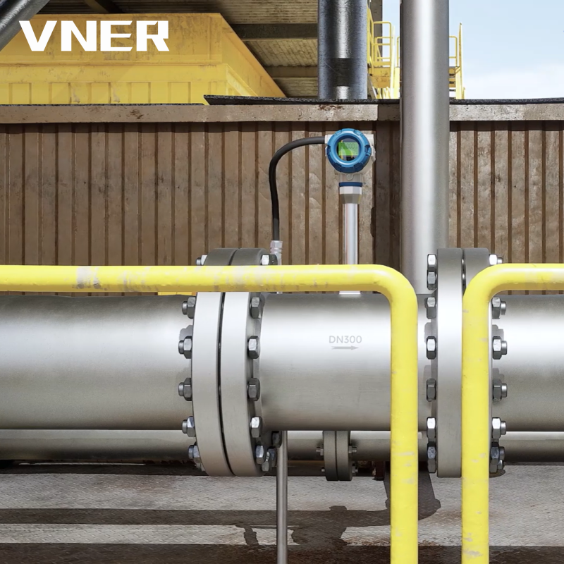 MA80T-TP Temperature/Pressure Compensated Vortex FlowmeterFor steam and gas metering where density compensation matters, it integrates RTD temperature and pressure input to output corrected volume or mass flow.View Product →
The MA80T series is a representative example of the vortex approach: the bluff body generates an alternating wake, the shedding frequency tracks velocity, and the meter outputs a frequency or pulse signal that is largely immune to zero drift. The trade-off is a minimum Reynolds number below which shedding stops being reliable, and a straight-run requirement upstream of the sensor.
Coriolis mass meters
Coriolis meters sidestep the entire argument. They measure mass flow directly from tube vibration, so density, temperature and pressure compensation become secondary rather than primary. If the process requirement is a mass balance, a custody transfer figure in kilograms, or a fluid whose density varies through the batch, a Coriolis meter removes a whole layer of assumptions. The cost is capital, pressure drop and size limits on large lines, but for the right application it is the shortest path to a defensible number. The operating principle is described in more depth in this explanation of how a Coriolis mass flow meter works.
Electromagnetic and turbine meters
Electromagnetic meters apply Faraday's law to a conductive liquid and produce a signal proportional to average velocity, independent of density, viscosity and, within limits, of the velocity profile. Turbine meters count rotor revolutions and are excellent on clean, low-viscosity liquids with steady flow. Both are velocity devices and both need a fully developed profile, which is a polite way of saying they need straight run and no swirl.
Density Is the Variable That Decides Whether Compensation Is Needed
Because dynamic pressure contains density linearly, any flow calculation built on dynamic pressure inherits the density error directly. A 5 percent density error produces a 5 percent flow error, with no ambiguity and no partial cancellation.
For liquids, density changes are small and often ignored, correctly. Water at 20 C is 998 kg per cubic metre and at 80 C is 972, a 2.6 percent difference. If the application tolerates 2 percent, no compensation is needed. If it is a custody transfer or an energy measurement, it is not optional.
For gases, density is proportional to absolute pressure and inversely proportional to absolute temperature. A gas line at 8 bar gauge swinging between 10 C and 40 C changes density by about 10 percent from temperature alone. Ignoring that is a 10 percent error in a flow reading that may be used to bill someone. The correct answer is pressure and temperature compensation at the point of measurement, either through a flow computer or through an integrated transmitter.
This is where purpose-built compensated instruments earn their price. A swirl meter with integrated temperature and pressure compensation measures the two variables that govern density, computes the corrected value, and outputs a standardised volume or mass figure without a separate compensating loop. Fewer field connections means fewer failure points, and the compensation is guaranteed to be applied with the same fluid properties used in the sizing calculation.
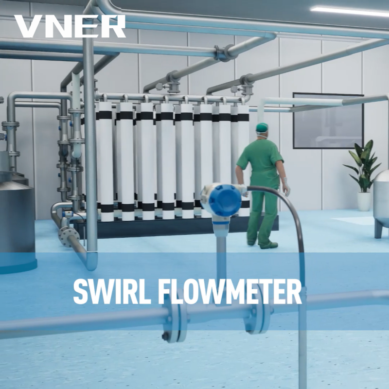 SA80T-TP Temperature/Pressure-Compensated Swirl FlowmeterBuilt-in temperature and pressure compensation supports standard volume or mass output for steam and gas metering with fewer external correction components.View Product →
The SA80TTP is an example of that approach: the temperature and pressure compensation is built into the device rather than bolted on downstream. For steam, compressed air and fuel gas, that integration is usually the difference between a number an auditor accepts and a number that needs a spreadsheet to defend.
Common Misconceptions Worth Retiring
- "Static pressure only exists when the fluid is stopped." Wrong. Static pressure is measured in the moving fluid, by a tap that does not face the flow.
- "Dynamic pressure pushes on the pipe wall." Not directly. Dynamic pressure is directional; the wall sees static pressure plus whatever the flow pattern imposes through friction and turbulence.
- "Total pressure is always higher than static." True for a stagnation point, but total pressure falls along a real pipe because of friction. Total pressure is conserved along a streamline only in the absence of losses.
- "A bigger differential pressure means a bigger flow." Only within the same element and the same fluid state. Change the orifice bore, the pipe diameter or the density, and the comparison is meaningless.
- "Velocity pressure readings can be averaged arithmetically across a duct." They can, and it is wrong in a non-uniform profile. Average the square roots to get mean velocity, then square the result for mean velocity pressure.
- "If the static pressure is stable, the flow is stable." Static pressure stability tells you about the system, not the flow. A control valve can hold pressure steady while flow swings 30 percent.
A Specification Checklist That Prevents Most of These Problems
Before a purchase order goes out, these questions should have written answers, not verbal ones.
- What is the fluid state at the meter: phase, density, viscosity, temperature range, pressure range, and whether any of these change during the batch?
- Is the required result a mass, a standard volume, an actual volume or a velocity? Each implies a different correction chain.
- What turndown is genuinely needed, and what accuracy is required at the bottom of that range rather than at the top?
- Which pressure is the instrument actually sensing, and is that the quantity the sizing calculation assumed?
- What straight run is available, and what does the manufacturer require? A 5D upstream allowance for a meter that needs 15D is a design change, not a commissioning fix.
- How will the reading be verified on site, and against what reference? A pitot traverse, a calibrated master meter, or a weighing system all have different uncertainties.
- What is the impulse line or tapping arrangement, and who is responsible for slope, venting and draining?
- For gas, is compensation integrated, panel-mounted or absent, and who signs off on the fluid properties used?
- What happens at zero flow, and what does the meter output? A live zero is useful; a silent 4 mA is not.
The engineering team behind the instrument matters as much as the datasheet here. A supplier who can show sizing calculations, calibration records and field experience across similar process conditions is worth more than a catalogue with a wider range. VNER, for example, has been building flow instrumentation since 2011 and describes its approach as engineering-driven sizing rather than catalogue selection, with in-house calibration and project delivery across more than 30 countries. Background on the company and its measurement portfolio is available on the company profile page, and it is the sort of context worth checking before a difficult application goes to tender.
The Numbers to Carry Away
Static pressure is the wall pressure. Dynamic pressure is half the density times the square of the velocity. Total pressure is the sum, and stagnation pressure is what you get when the flow is stopped at a probe tip.
For water at 3 m/s, expect about 4.5 kPa of dynamic pressure against a static pressure measured in bar. For air at 12 m/s, expect about 86 Pa against a static pressure measured in hundreds of pascals. The ratio between the two pressures tells you immediately whether a small differential measurement is viable, whether compensation is mandatory, and how much turndown the application can realistically support.
Most field failures in flow measurement are not instrument failures. They are mismatches between the pressure the sensor measures and the pressure the sizing calculation assumed. Sorting that out before the meter is ordered costs a short conversation. Sorting it out after commissioning costs a shutdown, a re-range and an uncomfortable meeting.


Products
Contact Information
-

+86 18652789521
+86-0514-83633600 / 83633900 -

+86-0514-83633600 / 83633900
-

s@vner.com.cn
katherine@vner.com.cn -

No. 11 Xingye Road, Chenji Town Industrial Park, Yizheng, Yangzhou, China
